

SADL Author Junhan Sun on Tracing the Origin of Representation Collapse in JEPA World Models
Researchers from Zhejiang University and Tsinghua University have introduced SADL, a training method that prevents representation collapse in Joint-Embedding Predictive Architecture (JEPA) world models by applying constraints directly to the visual encoder. The approach significantly improves multi-task training stability and control success rates in robotic simulations.

World models based on the Joint-Embedding Predictive Architecture (JEPA) encode images into internal representations, which are then used to predict future states.
The process of converting visual frames into numerical data is called "encoding," and the resulting set of numbers constitutes the frame's "representation."
If two distinct images yield nearly identical representations after encoding, the model struggles to make accurate judgments based on them. When many originally distinct frames are encoded into indistinguishable representations, "representation collapse" occurs.
To ensure the representations of different frames remain distinct, researchers typically introduce constraints during training. However, these constraints are applied to the output of the projection layer. The encoder first generates the representation, which the projection layer then processes. While the projection layer can recombine and amplify any residual differences in the representation, it cannot recover information that has already been lost. Consequently, even if the projection output satisfies the constraints, it does not guarantee that the encoder has retained sufficient information to distinguish between different frames.
If the projection layer's output still appears distinct, how could the encoder have already lost the information required to differentiate the frames?
On November 16, Junhan Sun of Zhejiang University served as the first author, with Hao Zhao, Assistant Professor at Tsinghua University, and Guofeng Zhang, Professor at Zhejiang University, as corresponding authors. The team, in collaboration with the State Key Laboratory of CAD&CG at Zhejiang University, the Institute for AI Industry Research at Tsinghua University, RoboParty Lab, Alibaba Group, and InSpatio, released the paper "SADL: On the Demand-Supply Geometry of Representation Collapse."
The study frames this discrepancy as a mismatch between the "demand" of the projection layer and the "supply" of the encoder, and introduces a training method called SADL: when the differences retained by the encoder are insufficient, constraints are applied directly to the encoder.
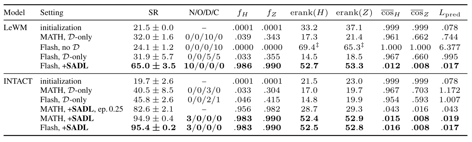
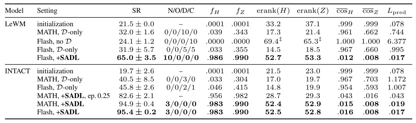
This work originated from issues encountered while the team was training INTACT, a robot world model, and was subsequently validated on another world model, LeWorldModel (LeWM). To observe the dynamics of representation collapse, the researchers trained LeWM using a FlashAttention backend and removed the original output constraints. After a single epoch of joint training across four tasks, the encoded representations of distinct frames were nearly identical, and the average success rate across the four tasks stood at 24.1%.
The work quickly gained attention after being posted on X. Within just one day, Junhan Sun's post introducing SADL garnered nearly a thousand likes and was retweeted and replied to by Yann LeCun, the originator of JEPA, who commented, "Nice." Junhan Sun subsequently responded that receiving affirmation from the creator of JEPA means a great deal to him.

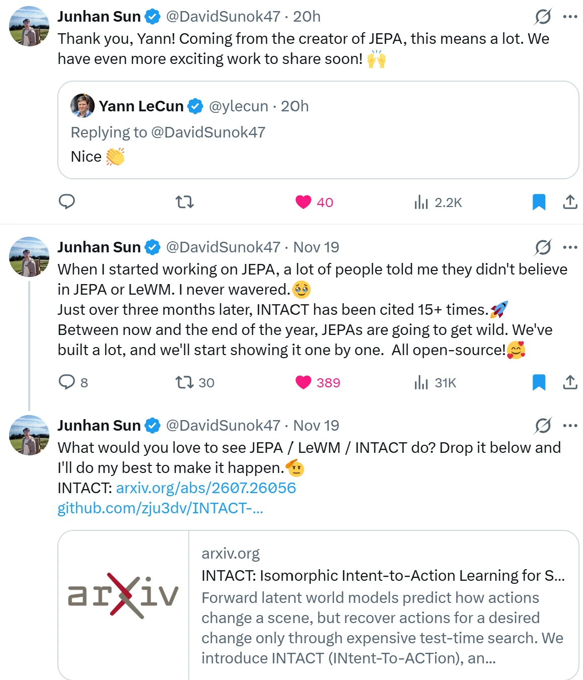
Coinciding with the paper's release, 42HOW Robotics interviewed the paper's first author, Junhan Sun. They discussed how the team pinpoints representation collapse, how to determine when the encoder needs correction, and how close these training advances are to deployment on real robots.
Representation collapse begins at the encoder
Junhan Sun recalls that the team began working on JEPA in May of this year and released the robot world model INTACT in late July. The project's experiments initially used a MATH-only backend for attention computation. While this approach was slower and consumed more VRAM, switching to other backends led to a critical issue: "whether in single-task or four-task training, representation collapse could occur." The team tried swapping out the regularization terms designed to prevent collapse, but the problem persisted. By August, they began systematically debugging the model components one by one.
To trace the origin of numerical discrepancies during training, the team fixed the initial parameters, input sequence, random state, and optimizer, swapping only the attention backends of the visual encoder and the predictor. When the encoder used MATH and the predictor used Flash, the first 100 steps across three experimental runs were bit-for-bit identical to the reference results. However, when the two were swapped, numerical discrepancies appeared at step one in all three runs. In one of these experiments, the earliest detected difference emerged in the gradients during the visual encoder's backpropagation, which then progressively amplified during parameter updates.
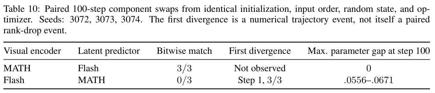
The numerical deviation at the first step provided a crucial clue for debugging. To pinpoint where the representation began to degrade, the researchers examined the outputs of each layer across 37 training runs. Thirteen of these runs exhibited severe degradation, with the effective rank dropping to less than half of the healthy reference value for that same training epoch; the earliest observed anomalies all occurred within the visual encoder. The effective rank reflects the number of effective directions across which the variations between samples are distributed. A decline in this metric indicates that the variations between different frames are increasingly concentrating along just a few directions.
"We ran several ablation experiments to figure out exactly where the collapse originates. We found that the final few layers of the encoder—specifically, the last few layers of the ViT—are the first to collapse," Junhan Sun said.
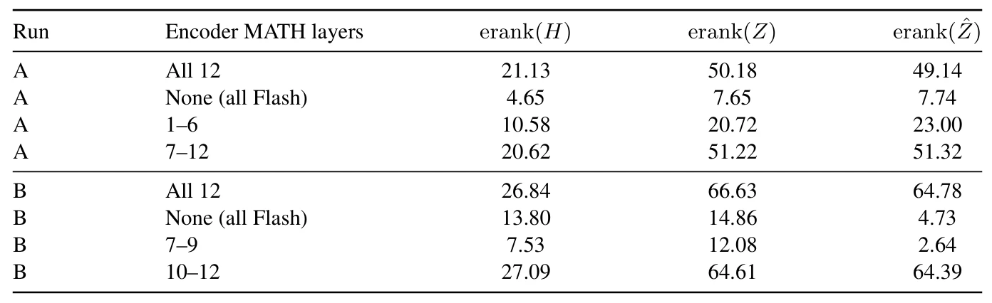
To determine which layers are most sensitive to the attention backend, the team fixed the predictor to MATH and varied only the layers using MATH within the encoder, subsequently measuring the representation using the same batch of PushT samples. When only layers 7 through 9 were swapped, the effective rank of the encoder's output was 7.53. When only the final layers 10 through 12 were swapped, the effective rank reached 27.09, closely approaching the 26.84 achieved when all 12 layers used MATH.
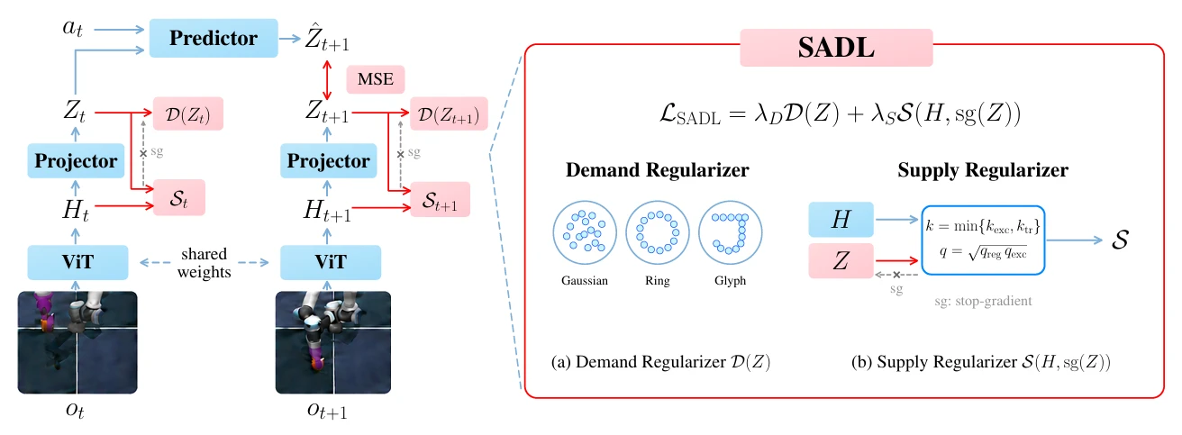
The encoder has already begun to degrade, so why didn't the original training constraints correct it in time? A single frame first passes through the visual encoder ViT to yield the representation H, and then through a projection layer to produce Z. The predictor takes the current Z and the action as inputs to predict the representation at the next time step. D(Z) in the figure represents the original anti-collapse constraint, which acts directly on Z. Changes within the encoder must propagate through the projection layer to potentially affect this constraint.
The team measured the sample differences preserved by LeWM and INTACT across the encoding and projection stages. At the start of training, the differences between different samples accounted for only about 0.01% of the total energy in the encoder representation. After just one epoch of training with the original output constraints, this proportion rose to approximately 3%–5% in H and about 30%–42% in Z. Taking INTACT with Flash as an example, sample differences accounted for 4.6% in H and 41.5% in Z. By subtracting the components common to a batch of images, the projection layer can increase the proportion of the remaining differences in its output.
To determine when this discrepancy emerges during training, the team compared the effective rank dynamics of the deep encoder layers and Z on LeWM. The experiments used Flash, applied only the SIGReg constraint to Z, and defined the threshold as the normalized effective rank dropping below 50% of its respective peak. Out of 40 "training run × task" combinations, Z dropped below the threshold in 16 cases. In 5 of these, the encoder dropped below the threshold earlier; in 7, both dropped below during the same recorded interval; and in the remaining 4, the encoder was already below the threshold from the very first measurement. Furthermore, in 5 additional combinations, only the encoder was observed to drop below the threshold. Monitoring Z alone would have missed these 5 instances of degradation.

The issue lies in what happens to the training signal as it passes through the projection layer. The projection layer used in the study incorporates batch normalization, which subtracts the mean of the samples within the same batch during training. If the exact same set of values is added to the encoding output of every image, the batch mean increases by that same amount, leaving Z unchanged after subtraction. Mathematically, the directions of these shared changes fall within the null space of the projector Jacobian. Consequently, neither the prediction loss computed via Z nor the anti-collapse constraint can propagate corrective signals back to H along this shared direction. The shared components can continue to dominate the energy in H, while the variations that actually distinguish different images are relegated to a tiny fraction.
The team also tested applying the constraints directly to the encoder. Both experimental setups used the same attention backend, altering only the location of the constraints. When constraining only Z, the effective rank of H was 4.65. When the constraint was shifted to H alone, this value increased to 27.90, the effective rank of Z was 9.67, and the effective rank of the predictor output dropped from 7.74 to 2.96. The sample differences in the encoder were distributed across more dimensions, whereas the differences in the predictor output became more concentrated.

This leaves two questions for subsequent methods: How much of the image difference is preserved in the encoder, and how much of it actually propagates to the projection output?
SADL constrains the encoder on demand
The team proposed SADL, which stands for Supply And Demand Loss. This training method retains the original prediction loss and projection layer constraints while adding an on-demand "supply regularization" term to the encoder. The additional constraint is activated only when the differences the encoder can retain and pass to the projection layer fall below the current demand.
"We supply exactly as much as the demand requires," Junhan Sun explained in the interview.
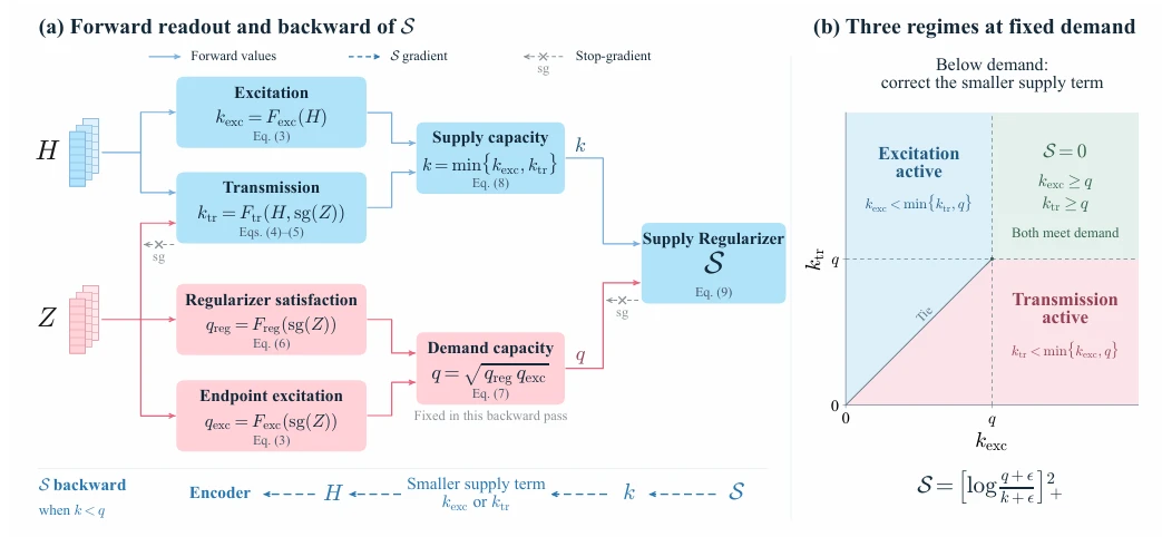
Specifically within the model, supply is determined by two scores. "Excitation" measures how much of the variation in H originates from different samples and across how many directions these differences are distributed. "Transmission" estimates how much of the variation in H can find a corresponding representation in Z, based on the linear correlation between H and Z. SADL takes the lower of these two scores as the supply, k. If either score falls short, it limits the actual supply.
The demand, q, is calculated from the current state of Z. The team uses one score to measure how well Z satisfies the original output constraints and another to measure the sample variance Z has already formed, taking the geometric mean of the two. During training, the model first calculates the demand from the current Z to serve as the reference for that update. When the supply falls below the demand, an additional correction signal is sent directly to the encoder, targeting the lower of the two supply scores. Once both scores meet the demand, the penalty drops to zero.
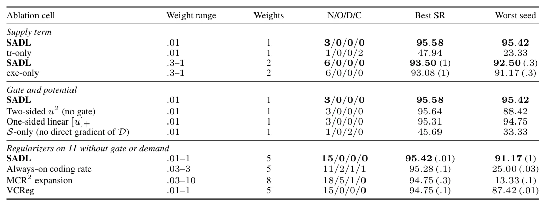
To test what issues excitation and transmission can each identify, the team fixed the demand at 0.70 and introduced two types of deficits. In the first set, existing sample differences could be transmitted, but the encoder retained too little variation. When monitoring only transmission, the excitation score remained at 0.494 after 200 steps, whereas the full SADL increased it to 0.713. In the second set, the encoder retained sufficient variation, but transmission could not keep up. When monitoring only excitation, the transmission score plateaued at 0.314, and the full SADL raised it to 0.789. In both sets of experiments, the individually monitored metric had already met its target, so the deficit in the other metric did not trigger any correction.
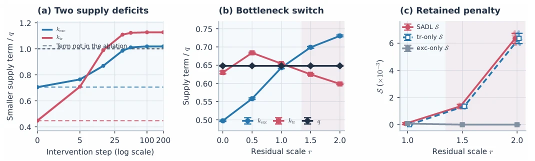
The team then evaluated the "stop when sufficient" rule during the four-task training in INTACT. The baseline used a bidirectional penalty, punishing the model whether the supply exceeded or fell short of the demand. Under identical weights, after one epoch of training, the average success rates for the bidirectional penalty and the full SADL were 95.64% and 95.58%, respectively. While the average performances of the two groups were similar, their worst-case runs differed by 7 percentage points, scoring 88.42% and 95.42%, respectively.
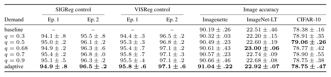
The demand can also be set to a fixed value. The team compared the approaches under two output constraints. When using SIGReg, after two epochs of training, the average four-task success rate was 96.8% with a fixed q=0.70, compared to 96.5% with adaptive demand. Switching to VISReg, a fixed q of 0.68, 0.70, or 0.90 all achieved 97.1%, and the adaptive demand also reached 97.1%. If chosen appropriately, a fixed value can yield comparable results. However, adaptive demand allows the model to apply the same rule set when switching to a new training configuration, calculating the demand directly from the current output.
SADL modifies only the training objective, leaving the model architecture and prediction pipeline unchanged. The true test in real-world robotic tasks is whether the variations preserved and transmitted to Z actually improve prediction accuracy, and whether those predictive gains translate into higher control success rates.
More stable representations and higher control success rates
What is the difference in outcomes when a single world model learns four tasks separately versus when a single encoder learns all four tasks simultaneously?
In an interview, Junhan Sun noted that his primary concern is whether JEPA can advance toward multi-task joint training once representation degradation is resolved. To investigate this, the team conducted two sets of experiments on LeWorldModel (LeWM) and INTACT. The single-task experiments trained PushT, Cube, Reacher, and TwoRoom separately and then averaged the results across the four tasks. In contrast, the joint training setup shared the encoder and projection layers across all four tasks. During evaluation, LeWM searches for candidate actions while INTACT outputs actions directly; therefore, performance gains are compared within each respective model.
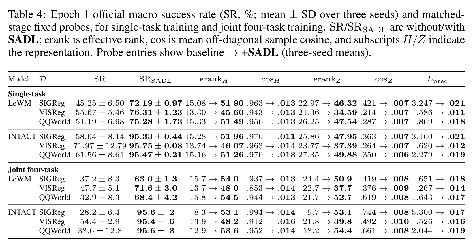
The team evaluated both models using three different output constraints. After one epoch of training, adding SADL to the six control groups in the single-task experiments improved the average success rate by 20.6 to 36.7 percentage points. In the six control groups for the four-task joint training, the improvement ranged from 23.9 to 67.4 percentage points. For example, in the joint training setup combining INTACT and SIGReg, the effective rank of the encoder output H increased from 8.3 to 53.1, and the effective rank of the projection output Z rose from 9.7 to 53.1. The loss for predicting the next state representation dropped from 5.300 to 0.017, while the average success rate across the four tasks surged from 28.2% to 95.6%. Within this same set of experiments, the diversity preserved by the encoder, the accuracy of the predictions, and the final control performance all improved.
While the average performance improved, would the representations still collapse from a different random initialization? To test this, the team repeated the four-task LeWM training using 10 random seeds, keeping the Flash backend and SIGReg output constraint fixed. After two epochs, among the 10 runs using only the original constraints, five experienced degradation and five collapsed. With SADL added, all 10 runs met the baseline standards set by the research. Reflecting on these results, Junhan Sun noted, "There was degradation and collapse before, but now there is neither." For joint training, these results highlight a critical factor that average success rates alone cannot reveal: whether the model can train stably across different random initializations.
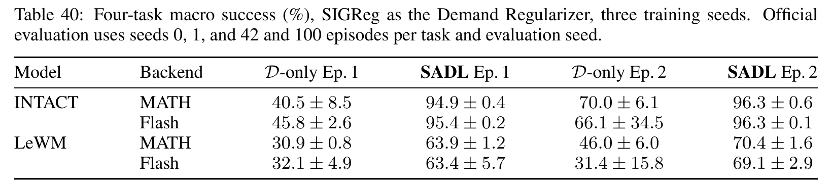
The team also isolated the attention backend, data ordering, and number of updates to verify whether the gains stemmed specifically from switching to the Flash backend. For INTACT, after two epochs of training, adding SADL with the MATH backend raised the four-task average success rate from 70.0% to 96.3%. With the Flash backend, it increased from 66.1% to 96.3%. LeWM showed similar improvements under both backends. Across all four control groups, training with SADL for just one epoch outperformed the baseline trained for two epochs on the same backend. For INTACT, these two training budgets correspond to 5,695 and 11,390 parameter updates, respectively.
Next, the team replaced the output constraints with different distribution targets. During training, the researchers tracked the four-task success rates across four settings, including a ring mixture distribution and a spherical shell distribution. Under the ring mixture distribution, INTACT with SADL reached a 97.8% success rate by the fifth epoch. To observe the impact of adding SADL to LeWM, readers can compare the red and gray lines within the same subplot, which correspond to the same model.
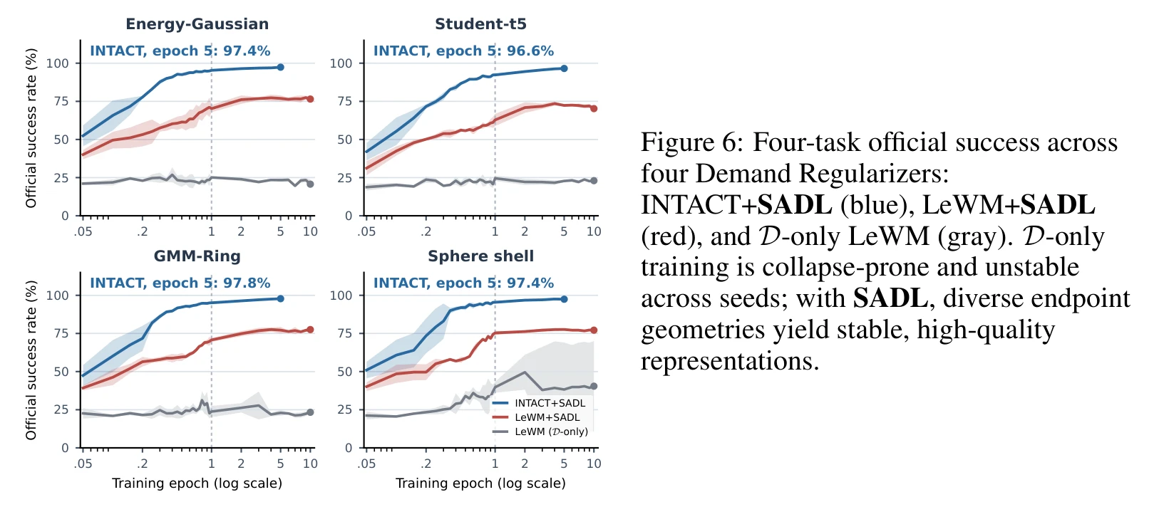
Aggregating the results across all eight output constraints, the four-task average success rate for INTACT after one epoch of training ranged from 92.33% to 95.81%, with seven of the settings exceeding 95%. However, a breakdown of the average scores reveals significant performance gaps between individual tasks. For instance, with SIGReg, the four-task average success rate was 95.58%, and both Cube and TwoRoom achieved 100% in this evaluation. In contrast, PushT, which requires pushing a T-shaped block into position and aligning its orientation, achieved only an 85.44% success rate. Across the eight settings, PushT's performance ranged between 76.67% and 86.33%.
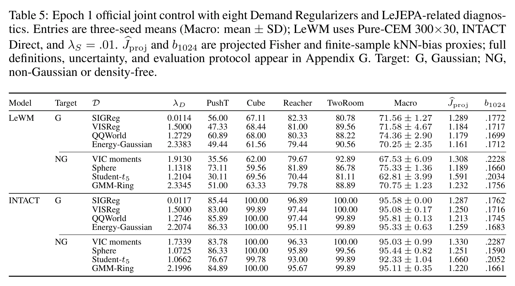
When all four tasks share a single encoder, SADL enables the model to reach higher average performance much earlier. The single-task results for PushT also demonstrate that even when the average success rate exceeds 95%, tasks requiring precise alignment of both position and orientation still have significant room for improvement.
From Image Classification to Real Robots: How Far Can SADL Go?
SADL was originally developed to address training challenges in robotic world models. If the task is switched to image classification, can it still help the encoder learn useful representations earlier?
The team selected four datasets for paired experiments. Each pair used identical data, model architectures, training configurations, and evaluation protocols, differing only in whether SADL was applied. When calculating the activation score, the researchers introduced an image-specific adjustment: they first averaged the representations derived from the same image under various crops and augmentations before measuring the differences between distinct images. In this way, the score reflects the degree of distinction between images.
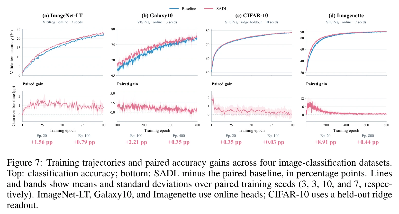
On ImageNet-LT and Galaxy10, the team used samples of dogs, birds, and galaxies to visualize the regions the model focuses on. They compared the representation distributions before and after applying SADL by projecting the samples onto a shared three-dimensional coordinate system. Classification accuracy was then used to evaluate how much class information these representations provide. At epoch 100 of ImageNet-LT training, the average accuracy with SADL reached 22.81%, compared to a baseline of 22.02%. For Galaxy10, SADL led by 2.21 percentage points at epoch 100, but the gap narrowed to 0.35 percentage points by epoch 400. Comparing these two time points reveals that part of the performance gain stems from the model learning to distinguish between classes earlier in training.
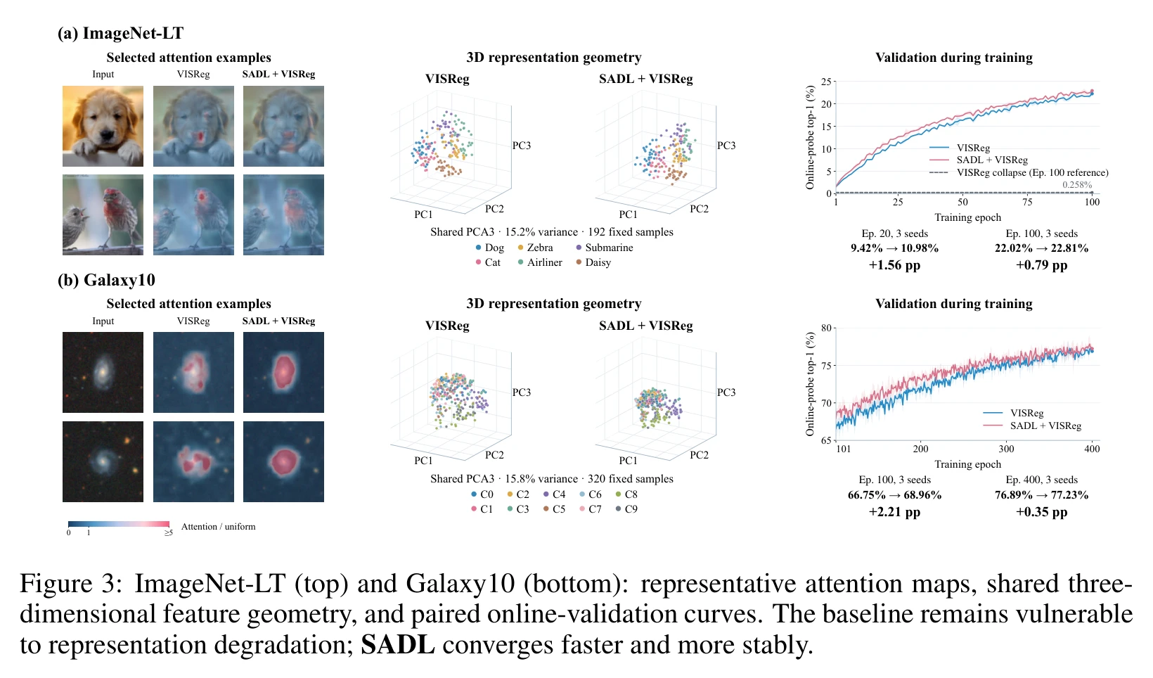
This "early acceleration, late convergence" trend is even more pronounced on the Imagenette dataset. At epoch 20, the model with SADL achieved an average accuracy of 44.51% compared to the baseline's 35.60%, with improvements across all seven paired training runs. By epoch 800, the gap between the two groups narrowed to 0.44 percentage points. On CIFAR-10, SADL also improved accuracy by 1.83 percentage points at epoch 1, but by epoch 100, the two groups reached 78.52% and 78.50%, respectively—a difference that falls within the variance of random seeds. The most consistent benefit across the image experiments is the early acquisition of representations suitable for classification. The final margin at the end of training depends on the specific dataset and training configuration.
During the interview, 42HOW Robotics also asked whether a model that has suffered from training collapse can be salvaged: "If a model is already ruined during training, can adding SADL midway still pull it back?"
"To be precise, there is a certain probability it can be recovered," Junhan Sun said.
The team selected training checkpoints that were close to collapse and had both groups resume training from the exact same checkpoint. Taking INTACT as an example, after resuming from the checkpoint with random seed 3072, the four-task average success rate for the group with SADL was 53.92%, compared to 24.42% for the control group. When switching to the checkpoint for seed 0, while still using a supply regularization weight of 0.01, the SADL group achieved 26.50%, falling below the control group's 28.92%. Because the starting points for these experiments still retained some sample variance, the recovery effect varied depending on the checkpoint and the strength of the constraint.
When it comes to real-world robot deployment, Junhan Sun believes JEPA's potential lies in System 0—the fast-reacting, low-level control layer. He values the model's ability to predict how actions will alter the state within the representation space, bypassing the need to reconstruct the full visual scene. By dedicating compute strictly to information that influences action, he sees an opportunity to build smaller, faster-responding models.
He also noted in the interview that the team is advancing the transition from simulation to real-world scenarios. While this study validates training stability and control in simulation, the System 0 concept still needs to be evaluated using response latency and task success rates on physical hardware.
Found an error? Tell us